Gradient Descent is one of the most basic and fundamental algorithms in machine learning. In this post I’ll attempt to explain how the algorithm works with Go code.
If you are completely new to the gradient descent algorithm, I’d suggest watching the Linear Regression with One Variable series of videos by Andrew Ng, he explains the theory behind the algorithm in great depth.
Motivation
If you’re a programmer like me, mathematical equations may not be intuitive and may even feel intimidating. I find that converting those equations to code helps me grasp them better and make them seem not as intimidating as before.
Gradient descent is one of the most fundamental algorithms used to find optimal parameters of machine learning models. In practice, you may rarely need to implement gradient descent on your own, however understanding how it works will help you better train complex ML models.
Note: These code examples are for educational purposes only and are in no way intended to be used in production.
Getting started
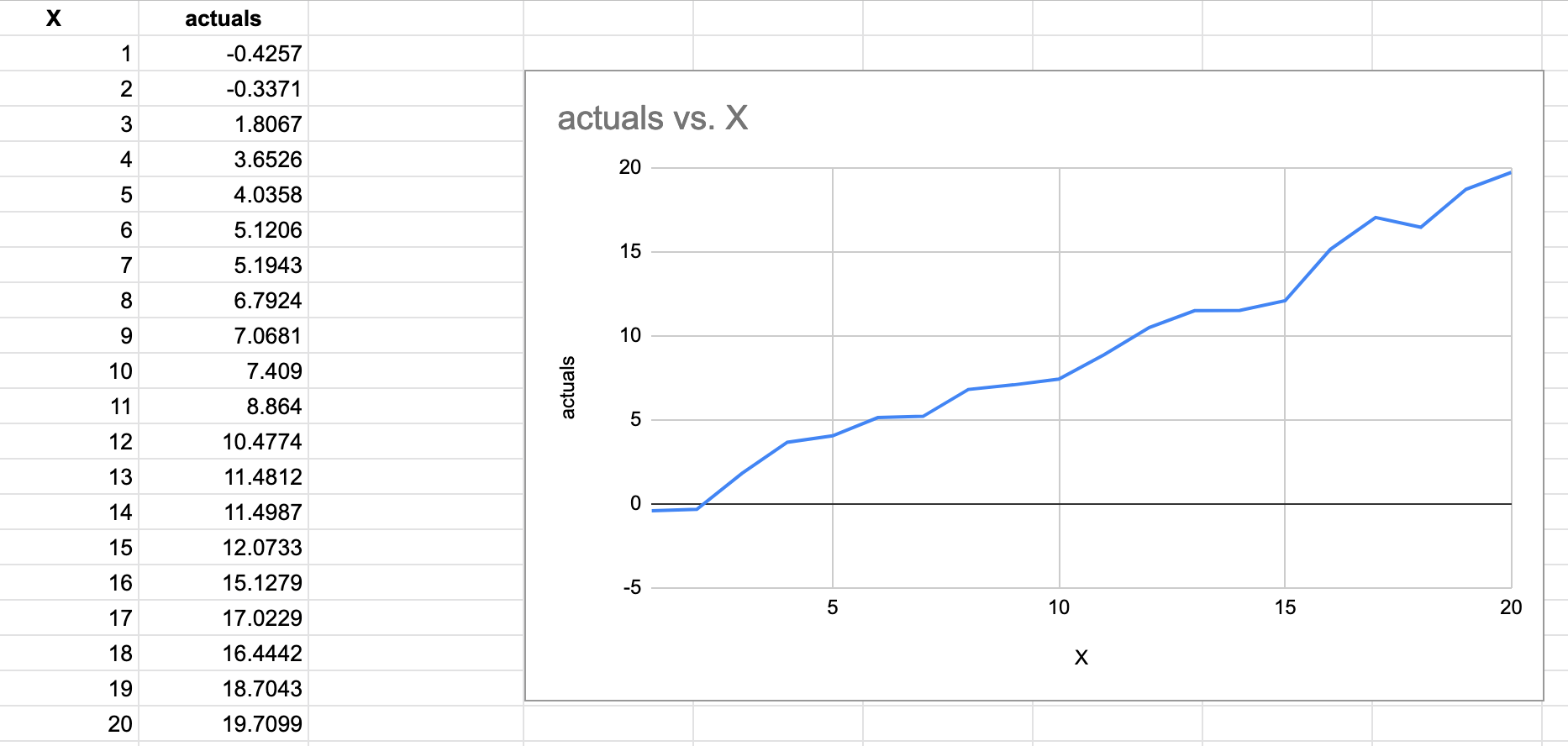
To get started, I’ve randomly generated points which approximately fall along a straight line. Hence for our model, we’ll use the straight line equation to predict points in the future.
Straight Line equation
y = mx + c // some countries may use the form y = mx + bThink of this as, our model needs to predict the value y given an input feature x. In order to do this we need to find the best values for m and c to fit the given sample values of x and y.
This is where the gradient descent algorithm comes in, we’ll use it to find the best possible values for m and c.
m and c are the parameters of our model.
The algorithm
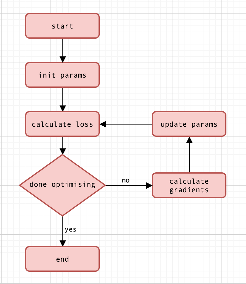
The model
Let’s start by defining our model with a function.
\[ f(x) = mx + c \]
1
2
3
4
5
6
7
8
9
10
11
12
13
14
15
16
var input_x = []float64{0., 1., 2., 3., 4., 5., 6., 7., 8., 9., 10., 11., 12., 13., 14., 15., 16., 17., 18., 19.}
var actuals = []float64{-0.4257, -0.3371, 1.8067, 3.6526, 4.0358, 5.1206, 5.1943, 6.7924, 7.0681, 7.4090, 8.8640, 10.4774, 11.4812, 11.4987, 12.0733, 15.1279, 17.0229, 16.4442, 18.7043, 19.7099}

type params struct {
	m float64
	c float64
}

// Equation for a straight line i.e y = mx + c or y = mx + b
func f(x []float64, p *params) []float64 {
	var result []float64
	for _, val := range x {
		y := p.m*val + p.c
		result = append(result, y)
	}
	return result
The loss function
We need a way to measure how good or bad values of m and c are. To do this we need to define a loss function J.
We’ll use the mean squared error (MSE) loss function, which is the mean of squared difference between predicted and actual values.
\[ J = \frac{1}{n}\displaystyle\sum_{i=0}^{n-1} \big(f(x[i]) - y[i] \big)^2 \] \[ \text{ where n is the size of the input} \]
1
2
3
4
5
6
7
8
9
10
// MSE or Mean Squared Error
func costFunction(predictions []float64) float64 {
	var diff float64
	for i := range actuals {
		d := predictions[i] - actuals[i]
		diff += math.Pow(d, 2.0)
	}
	loss := diff / float64(len(actuals))
	return loss
}
Calculating the gradients
Our objective with gradient descent is to minimize the loss (or cost) function.
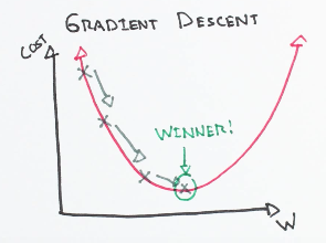
The image above represents the graph of a loss (or cost) function with a single parameter w. In order to know the direction to move in to get to the bottom of the curve, we calculate the gradient (or derivate or slope) at that point.
For our loss function J defined above, since we have two parameters, we have to compute the partial derivate w.r.t m and the partial derivate w.r.t c. The final values come out to be:
\[ \frac{\partial J}{\partial m} = \frac{2}{n}\displaystyle\sum_{i=0}^{n-1} \big(f(x[i]) - y[i] \big)x[i] \]
\[ \frac{\partial J}{\partial c} = \frac{2}{n}\displaystyle\sum_{i=0}^{n-1} \big(f(x[i]) - y[i] \big) \]
1
2
3
4
5
6
7
8
9
10
11
12
13
14
15
func calcGradientM(predicted []float64) float64 {
	var diff float64
	for i, x := range input_x {
		diff += (predicted[i] - actuals[i]) * x
	}
	return (diff / float64(len(input_x))) * 2
}

func calcGradientC(predicted []float64) float64 {
	var diff float64
	for i := range actuals {
		diff += (predicted[i] - actuals[i])
	}
	return (diff / float64(len(actuals))) * 2
}
Updating the parameters
Once we know in which direction to move along the curve, we need to decide how big a step we need to take. Taking too big or too small a step will cause problems- to know more please refer to Andrew Ng’s videos above which gives an in-depth explanation.
The amount we step is controlled by the learning rate (LR).
\[ m_{new} = m_{old} - LR * \text{ Gradient of m} \] \[ c_{new} = c_{old} - LR * \text{ Gradient of c} \]
1
2
3
4
5
const lr = 1e-3
func updateParams(p *params, gradientM float64, gradientC float64) {
	p.m -= lr * gradientM
	p.c -= lr * gradientC
}
Putting it all together
In machine learning, an epoch is defined as one iteration of training though the dataset. Here we’ll set epochs = 15 and a learning rate of 1e-3. We then initialize the parameter with random values and start training.
Note: rand.Seed(7.0) is used to get reproducible results.
1
2
3
4
5
6
7
8
9
10
11
12
13
14
15
16
17
18
19
20
21
22
23
24
25
26
27
28
29
30
31
32
33
34
35
36
const (
lr = 1e-3
epochs = 15
)
func calculateLoss(x []float64, p *params) (loss float64, predicted []float64) {
predicted = f(x, p)
loss = costFunction(predicted)
return
}
func calculateGradients(predicted []float64) (gradM float64, gradC float64) {
gradM = calcGradientM(predicted)
gradC = calcGradientC(predicted)
return
}
func fit(p *params) {
loss, preds := calculateLoss(input_x, p)
fmt.Printf("Loss: %f m: %f c:%f", loss, p.m, p.c)
fmt.Println()
gradM, gradC := calculateGradients(preds)
updateParams(p, gradM, gradC)
}
func train(p *params, epochs int) {
for i := 0; i < epochs; i++ {
fit(p)
}
}
func main() {
rand.Seed(7.0)
p := ¶ms{m: rand.Float64(), c: rand.Float64()}
train(p, epochs)
}
Running this gives me the following results:
1
2
3
4
5
6
7
8
9
10
11
12
13
14
15
Loss: 1.034384 m: 0.918892 c:0.231507
Loss: 0.956183 m: 0.928337 c:0.231757
Loss: 0.911916 m: 0.935444 c:0.231827
Loss: 0.886815 m: 0.940794 c:0.231762
Loss: 0.872540 m: 0.944824 c:0.231596
Loss: 0.864379 m: 0.947862 c:0.231353
Loss: 0.859671 m: 0.950154 c:0.231053
Loss: 0.856914 m: 0.951885 c:0.230710
Loss: 0.855259 m: 0.953196 c:0.230335
Loss: 0.854226 m: 0.954190 c:0.229935
Loss: 0.853545 m: 0.954946 c:0.229518
Loss: 0.853063 m: 0.955523 c:0.229087
Loss: 0.852693 m: 0.955965 c:0.228646
Loss: 0.852387 m: 0.956307 c:0.228197
Loss: 0.852117 m: 0.956573 c:0.227743
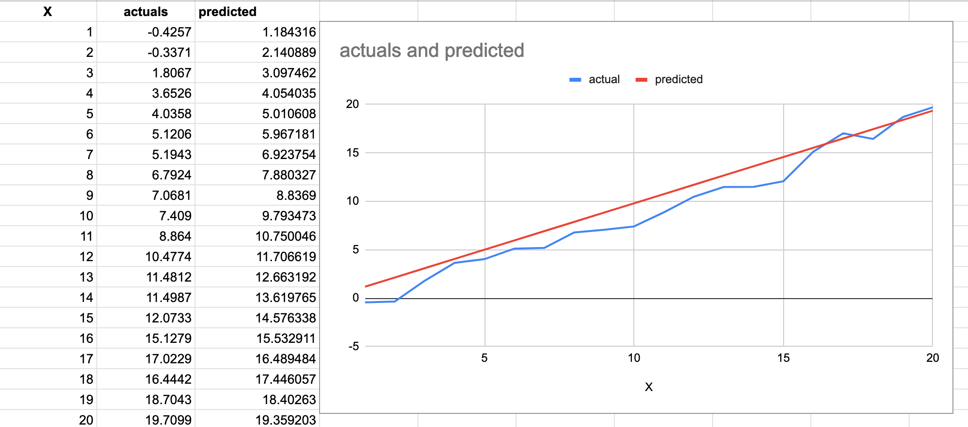
Plugging in the last values of m and c and plotting the resultant line on a graph along with the actual values give us this result.
Source Code
All the source code can be found on Github.