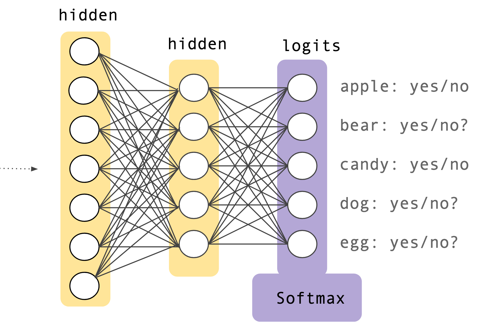
The softmax activation function is commonly used as the output layer in a neural network.
The Math
Mathematically, the softmax function is represented as follows.
\[ \Large\sigma(z_i) = \huge\frac{e^{z_i}}{\sum_{j=1}^{K}e^{z_j}} \]
For i = 1,…,K, K is the number of distinct classes to be predicted and z denotes the input vector.
For e.g. \[ \begin{bmatrix} 2.0 \\ 4.3 \\ 1.2 \\ -3.1 \end{bmatrix} \Rightarrow \begin{bmatrix} e^{2.0}/(e^{2.0}+e^{4.3}+e^{1.2}+e^{-3.1}) \\ e^{4.3}/(e^{2.0}+e^{4.3}+e^{1.2}+e^{-3.1}) \\ e^{1.2}/(e^{2.0}+e^{4.3}+e^{1.2}+e^{-3.1}) \\ e^{-3.1}/(e^{2.0}+e^{4.3}+e^{1.2}+e^{-3.1})\end{bmatrix} = \begin{bmatrix} 0.08749 \\ 0.87266 \\ 0.03931 \\ 0.00029 \end{bmatrix} \]
Why
The softmax activation function is often the final layer in multi-class classification neural networks. This function possesses the following important properties:
Ensure activations are positive numbers
It can be hard to interpret activation with negative values, taking the exponent ensure all values are positive.
Amplify small differences between activations
Taking the exponent also serves to amplify the difference between activations, this assists in picking one class over another.
Generate a valid probability distribution
Once we have positive values, normalizing across these values will generate activation between 0 and 1 which sum up to 1 and may be interpreted as probabilities.
Examples
Let’s validate our reasoning of the properties mentioned above. Consider the following activations.
\[ \begin{bmatrix} -0.1849 \\ 3.1026 \\ 1.7967 \end{bmatrix} \] It isn’t clear which class the input likely belongs to, let’s try to fix this by normalizing.
\[ \begin{bmatrix} -0.1849 \\ 3.1026 \\ 1.7967 \end{bmatrix} \Rightarrow \begin{bmatrix} -0.1849/(-0.1849+3.1026+1.7967) \\ 3.1026/(-0.1849+3.1026+1.7967) \\ 1.7967/(-0.1849+3.1026+1.7967)\end{bmatrix} = \begin{bmatrix} -0.0392 \\ 0.6581 \\ 0.3811 \end{bmatrix} \] Our activations now sum to 1, however we still have the first activation with a negative value of -0.0392 and hence regarding them as probabilities would be incorrect.
Finally, after applying the softmax function we end up with \[ \begin{bmatrix} 0.0285 \\ 0.7643 \\ 0.2070 \end{bmatrix} \]
The code
Note: These code examples are for educational purposes only and are in no way intended to be used in production.
We’ll be extending the concepts explained in my previous post on “Gradient descent with code” with matrix operations, considering an oversimplified neural network with a single linear layer. This should give you the intuition of what the activations look like, with and without using the softmax layer.
Note: We’ll be using the gonum library to represet our matrices and perform operations on them.
Putting it all together
Here SimpleNN() is an oversimplified representation of a neural network with a single linear layer and SoftMaxNN() is the network with the softmax layer.
1
2
3
4
5
6
7
8
9
10
11
12
13
14
15
16
17
18
func main() {
	SimpleNN()
	SoftmaxNN()
}

func SimpleNN() {
	nn := linear()
	fmt.Println("Activation after linear layer")
	fmt.Println(mat.Formatted(nn))
}

func SoftmaxNN() {
	nn := linear()
	nnsmax := softmax(nn)

	fmt.Println("Activation after softmax layer")
	fmt.Println(mat.Formatted(nnsmax))
}
Output
You should see an output similar to the one below.
Activations after linear layer \[ \begin{bmatrix} -0.971289832017899 \\ -0.31566700629829314 \\ 0.20609785706914163 \end{bmatrix} \]
Activations after softmax layer \[ \begin{bmatrix} 0.9849108426709876 \\ 0.013460649878849347 \\ 0.0016285074501629477 \end{bmatrix} \]
Linear Layer
Let’s code out the simple linear layer. In keeping with the conventions from the previous post, we’ll use m, x and c to represent our weights, inputs and biases.
To keeps things simple, we’ll assume we have only 3 classes which need to be predicted, hence our output matrix should have a dimension of 3x1.
Accordingly well assume m to have dimensions 3x3 and c to have 3x1.
E.g. mx + c
\[ \begin{bmatrix} 5 & 3 & 5 \\ 3 & 7 & 0 \\ 1 & 2 & 5 \end{bmatrix} \begin{bmatrix} 1 \\ 2 \\ 1 \end{bmatrix} + \begin{bmatrix} 1 \\ 1 \\ 1 \end{bmatrix} = \begin{bmatrix} 17 \\ 18 \\ 11 \end{bmatrix} \]
1
2
3
4
5
6
7
8
9
10
11
12
13
14
15
16
17
18
19
20
21
22
23
import "gonum.org/v1/gonum/mat"

func initRandomMatrix(row int, col int) *mat.Dense {
    size := row * col
    arr := make([]float64, size)
    for i := range arr {
        arr[i] = rand.NormFloat64()
    }

    return mat.NewDense(row, col, arr)
}

func linear() *mat.Dense {
    m := initRandomMatrix(3, 3)
    x := initRandomMatrix(3, 1)
    c := initRandomMatrix(3, 1)

    ll := mat.NewDense(3, 1, nil)
    ll.Mul(m, x)
    ll.Add(ll, c)

    return ll
}
initRandomMatrix is a helper method to initialize a matrix with random values.
Softmax Function
1
2
3
4
5
6
7
8
9
10
11
12
13
14
15
16
17
import "gonum.org/v1/gonum/mat"

func softmax(matrix *mat.Dense) *mat.Dense {
    var sum float64
    // Calculate the sum
    for _, v := range matrix.RawMatrix().Data {
	    sum += math.Exp(v)
    }

    resultMatrix := mat.NewDense(matrix.RawMatrix().Rows, matrix.RawMatrix().Cols, nil)
    // Calculate softmax value for each element
    resultMatrix.Apply(func(i int, j int, v float64) float64 {
	    return math.Exp(v) / sum
    }, matrix)

    return resultMatrix
}
As you can see from the code above, the softmax function is pretty straight forward.
Source Code
All the source code can be found on Github.